Note
These notes are taken after the fact based on the slides. Anything mentioned only in lecture is not included. Starting from
1-Introduction to Analysis, slide 1.
Why Take This Course?
- learn methods to improve software quality
- reliability, security, performance
- become a better software developer/tester
- build specialized tools for software diagnosis & testing
- for the war stories (real-world failures)
Case Study: Ariane Rocket Disaster (1996)
- caused by a numeric overflow error
- 64-bit sideways velocity stored in 16-bit space
- overflow misinterpreted as signal to change course
- cost:
- hundreds of millions of dollars
- multi-year setback to Ariane program
- video link
- post mortem
Security Vulnerabilities
- exploits of errors in programs
- examples:
- Moonlight Maze (1998)
- Code Red (2001)
- Titan Rain (2003)
- Stuxnet (2010)
- modern issues:
- malware on Android (2011 report: 0.5–1M users affected)
- 3/10 Android users face web-based threat yearly
- attackers = increasingly sophisticated
What is Program Analysis?
- program analysis = body of work to discover useful facts about programs
flowchart LR
    A[Program Analyzer A] --> B[Program P]
    B -->|works correctly| C[OK]
    B -->|fails for some inputs| D[Bug]
Examples of Program Issues
// Dead Code Example
public class DeadCode {
  public static void main(String[] args) {
    System.out.println("Hello World");
    return;
    System.out.println("This is dead code"); // never runs
  }
}

// Intentional Memory Leak
public class MemoryLeak {
  public static void main(String[] args) {
    while (true) {
      Integer[] arr = new Integer[1000]; // no release
    }
  }
}
Facts About Programs (1)
- Memory leaks → allocated but never freed
- Dead code → never executed
- Concurrency issues → race conditions / deadlocks
- Input validation → e.g., prevent SQL injection, XSS
- Code complexity → cyclomatic complexity (maintainability)
Facts About Programs (2)
- API misuse → wrong usage = subtle bugs
- Resource utilization → inefficient CPU/disk
- Type errors → mismatches (esp. in weakly typed languages)
- Uninitialized variables → undefined behaviour
- Exception handling → paths where exceptions may go unhandled
Other Interesting Questions
- does the program terminate on all inputs?
- how large can the heap become?
- can sensitive info leak to untrusted users?
- can untrusted users affect sensitive info?
- are buffer overruns possible?
- data races? SQL injection? XSS?
Program Points & Invariants
- program point: any value of program counter (any line of code)
- invariant: property that holds at a program point across all inputs/executions
foo(p, x) {
  var f, q;
  if (*p == 0) { f = 1; }
  else {
    q = alloc 10;
    *q = (*p) - 1;
    f = (*p) * (x(q, x));
  }
  return f;
}
Questions:
- will x be read later?
- can pointer p be null?
- which vars can p point to?
- is x initialized before read?
- lower/upper bounds on x?
- do p and q point to disjoint heap structures?
- can an assert fail here?
Why These Answers Matter
- efficiency: optimize resources
- correctness: verify behaviour & catch bugs
- program understanding
- enable refactoring
Types of Program Analysis
- Static analysis → compile-time, inspects code
- Dynamic analysis → run-time, monitors execution
- Hybrid → combines both
Static Analysis
- infers facts from code without execution
- tools/examples:
- Lint, FindBugs, Coverity (error patterns)
- Microsoft SLAM (API usage rules)
- Facebook Infer (memory leaks)
- ESC/Java (verify invariants)
Quiz: Program Invariants
int p(int x) { return x * x; }

void main() {
  int z;
  if (getc() == 'a')
    z = p(6) + 6;
  else
    z = p(-7) - 7;
}
At the end of the program, the value of z is always the same no matter which branch executes.
Question
- If the condition is true,
z = 6*6 + 6 = 42.- If the condition is false,
z = (-7)*(-7) - 7 = 42.- Therefore, the invariant at the end of the program is z == 42.
- The constant
cis 42.
Discovering Invariants (Static Analysis)
- some invariants are definitely true (e.g., z == 42)
- some are maybe invariants
- some are definitely not invariants
Dynamic Program Analysis
- infers facts by monitoring actual executions
- tools/examples:
- Purify (array bound checking)
- Eraser (data race detection)
- Valgrind (memory leaks)
- Daikon (likely invariants)
Anatomy of a Static Analysis
Key components:
- Intermediate Program Representation → CFGs, ASTs, bytecode
- Abstract domain → approximate states
- Transfer functions → update state per statement
- Fixed-point algorithm → iterative approximation until states stop changing
Terminology
- control-flow graph (CFG)
- abstract vs concrete states
- termination
- completeness
- soundness
Control Flow Graphs (CFGs)
- directed graph of program flow
- nodes = statements
- edges = control flow
- has one entry + one exit
- predecessor nodes = pred(v), successor nodes = succ(v)
flowchart TD
    A[start] --> B[f=1]
    B -->|n>0| C[f=f*n]
    C --> D[n=n-1]
    D --> B
    B -->|false| E[return f]
CFG Construction
A Control Flow Graph (CFG) models all possible paths of execution in a program. You build it inductively from the code:
- Simple statements (assignment, declaration, return, output) → one node each.
- Sequence
S1; S2;→ connect the exit ofS1to the entry ofS2. - Conditional (
if ... else ...) → one decision node with two outgoing edges: true and false; both rejoin after their subgraphs. - Loops (
while,for) → a decision node whose true edge enters the body and whose false edge exits the loop; the body flows back to the decision node, forming a cycle. - Entry/Exit → every CFG has a single entry and a single exit (they can be no-ops).
Simple Statements
flowchart LR
    A[entry] --> S[x = y + 1]
    S --> E[exit]
flowchart LR
    A[entry] --> S1[x = 0]
    S1 --> S2[y = x + 7]
    S2 --> E[exit]
flowchart TD
    A[entry] --> C{c}
    C -->|true| S1[x = x + 1]
    C -->|false| S2[x = x - 1]
    S1 --> J[join]
    S2 --> J
    J --> E[exit]
flowchart TD
    A[entry] --> C{c}
    C -->|true| B[body S]
    B --> C
    C -->|false| E[exit]
Normalization
- break complex expressions into single steps
- use fresh variables
x = f(y+3)*5;
// normalized
t1 = y+3;
t2 = f(t1);
x = t2*5;
Example Static Analysis Problem
- goal: find vars with constant values at program points
- method:
- draw CFG
- apply iterative approximation
Iterative Approximation
- method: start with guess → refine repeatedly until fixed point
- used for constant propagation, etc.
flowchart TD
    A[z=3] --> B{while true}
    B -->|x==1| C[y=7]
    B -->|else| D[y=z+4]
    C --> E[assert y==7]
    D --> E
    E --> B
Iterative Approximation Quiz
b = 1;
while (true) {
  b = b + 1;
}- what does analysis infer for b at:
- loop header
- entry of loop body
- exit of loop body
Solution
- loop header: b = ?
- entry: b = 1
- exit: b = ?
Overview of Static Analysis
- representation: CFG, AST, bytecode
- abstract domain: approximate states
- transfer function: how statements affect abstract state
- fixed-point algorithm: converge to stable state
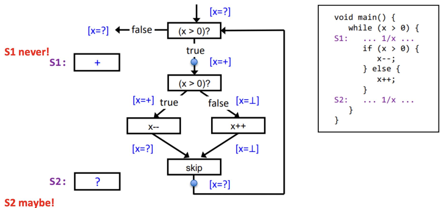
Quiz: Divide-by-Zero Example
- draw CFG
- analyze with iterative approximation
- classify statements:
- never divides by zero
- may divide by zero
Solution
Trade-offs in Software Analysis
- Static analysis
- proportional to program size
- sound (no false positives) but often incomplete
- Dynamic analysis
- proportional to execution time
- complete for observed runs but not sound (may miss bugs)