COSC 3P93: Lecture 10 Notes

Performance

Note

Starting at l4a.pdf, slide 10

Performance and Scalability

• Sequential runtime ($T_{seq}$): a function of problem size and architecture
• Parallel runtime ($T_{par}$): a function of problem size, parallel architecture, & number of processors used in the execution
  • Parallel performance affected by algorithm & architecture
• Scalability: how the program behaves in terms of complexity and system size (number of processors)
  • Strongly scalable: same efficiency when increasing system size when problem size does not change
  • Weakly scalable: same efficiency when increasing system size at the same rate as problem size

Performance metrics and formulas

• $T_1$: the execution time on a single processor
• $T_p$: the execution time on a N-processor system
• $S(p)=\frac{T_1}{T_p}$ (speedup)
• $E(p)=\frac{S_p}{N}=\frac{\frac{T_{seq}}{T_{par}}}{N}=\frac{T_{seq}}{{N.T}_{par}}$ (efficiency)
• $C(p)=p\ast T_p$

Speedups and efficiency

Parallel program

p	1	2	4	8	16
S	1.0	1.9	3.6	6.5	10.8
$E=S/p$	1.0	0.95	0.90	0.81	0.68

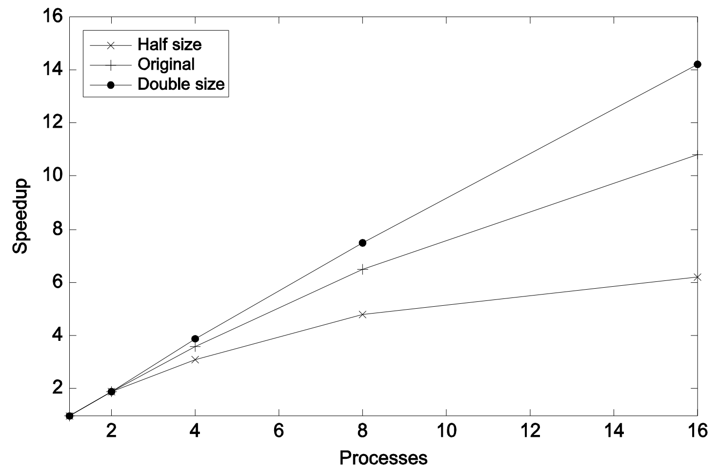Parallel program on different problem sizes

	p	1	2	4	8	16
Half	S	1.0	1.9	3.1	4.8	6.2
	E	1.0	0.95	0.78	0.60	0.39
Original	S	1.0	1.9	3.6	6.5	10.8
	E	1.0	0.95	0.90	0.81	0.68
Double	S	1.0	1.9	3.9	7.5	14.2
	E	1.0	0.95	0.98	0.94	0.89

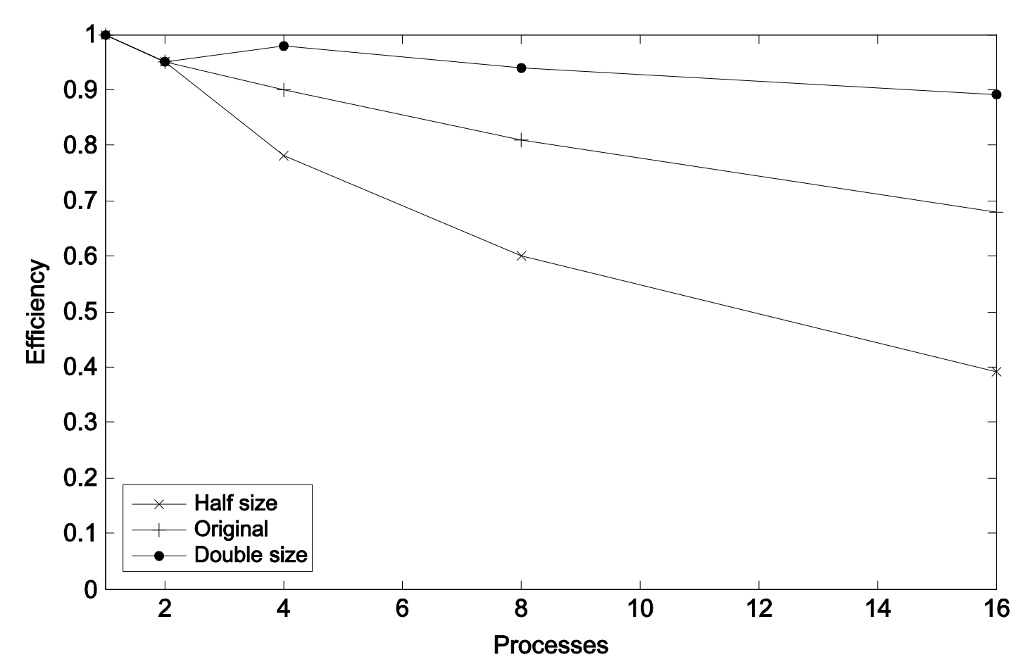Limits & costs of parallel programming

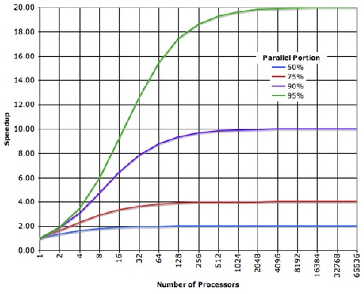
Amdahl’s law

• potential program speedup is defined by the fraction of code ($P$) that can be parallelized

$$speedup=\frac{1}{1-P}$$

• if none of the code can be parallelized → $P=0$ and $speedup=0$ (no speedup)
• if all of the code is parallelized → $P=1$ and $speedup=\infty$ (in theory)
• if 50% of the code can be parallelized → maximum speedup $=2$ (code will run twice as fast)

N	P = 0.50	P = 0.90	P = 0.95	P = 0.99
10	1.82	5.26	6.89	9.17
100	1.98	9.17	16.80	50.25
1000	1.99	9.91	19.62	90.99
10000	1.99	9.91	19.96	99.02
100000	1.99	9.99	19.99	99.90

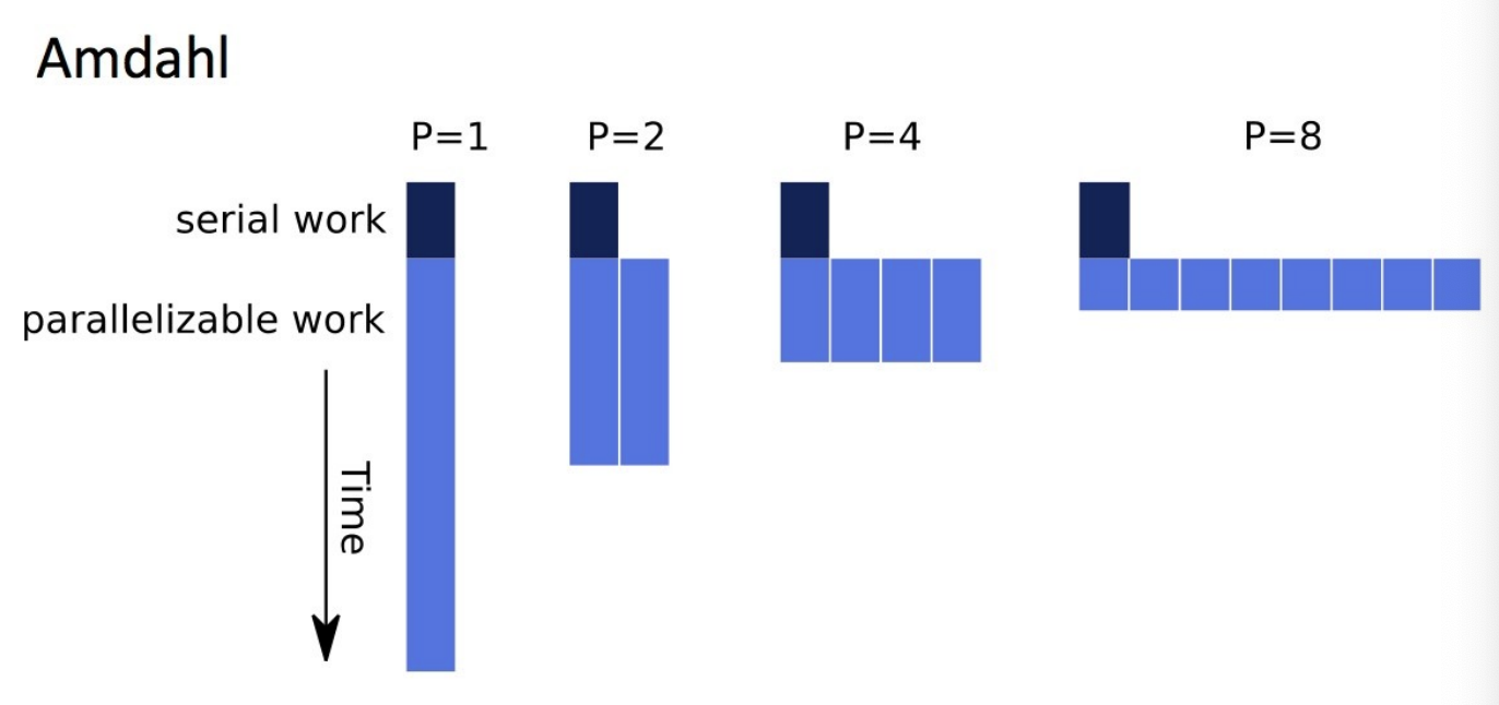
Amdahl’s law - Fixed size speedup

• Let $S$ be the fraction of a program that is sequential → $1-S$ is the fraction that can be parallelized
• Let $T1$ be the execution time on 1 processor
• Let $Tp$ be the execution time on N processors
• $Sp$ is the speedup

$$\begin{gathered} Sp=\frac{T_1}{T_p} \\ =\frac{T_1}{(S\cdot T_1+(1-S)\cdot \frac{T_1}{N})} \\ =\frac{1}{S+\frac{(1-S)}{N}} \end{gathered}$$

• As $N\to \infty$

$$Sp=\frac{1}{S}$$

• When does Amdahl’s Law apply?
  • when the problem size is fixed
  • strong scaling ($N\to \infty$, $Sp\to S_{\infty }=1/S$)
  • speedup bound is determined by the degree of sequential execution time in the computation, not # of processors

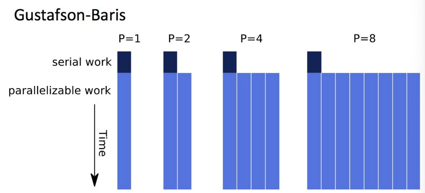
Gustafson-Barsis’ Law (scaled speedup)

• assume parallel time is kept constant
  • $Tp$ is constant
  • $P_{seq}$ is the fraction of $T_p$ spent in sequential execution
  • $P_{par}$ is the fraction of $T_p$ spent in parallel execution
• What is the execution time on one processor?

$$T_s=P_{seq}\ast Tp+(1-P_{seq})\ast N\ast Tp$$

• What is the speedup in this case?

$$\begin{gathered} S_p=\frac{T_s}{T_p} \\ =\frac{(P_{seq}\cdot T_p+(1-P_{seq})\cdot N\cdot T_p)}{T_p} \\ =P_{seq}+(1-P_{seq})\cdot N \\ =(1-P_{par})+P_{par}\cdot N \end{gathered}$$

• When does Gustafson’s Law apply?
  • when problem size can increase as the number of processors increases
  • weak scaling ($Sp=P_{seq}+N{P}_{par}$)
  • speedup function includes number of processors
  • can maintain or increase parallel efficiency as the problem scales

Amdahl vs Gustafson-Baris

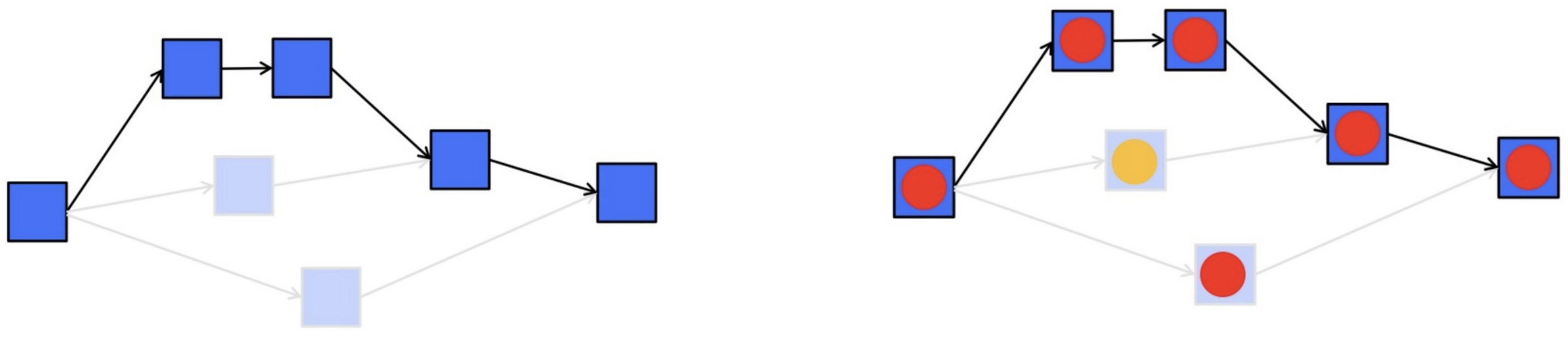
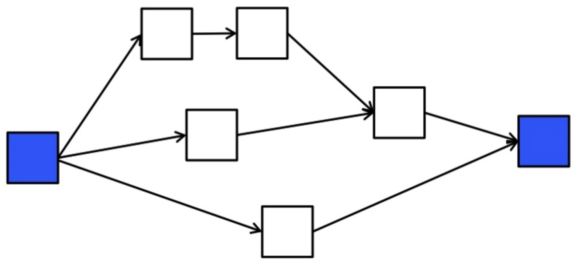
DAG Model of Computation

• think of a program as a directed acyclic graph (DAG) of tasks
  • task cannot execute until all the inputs to the task are available
  • these come from outputs of earlier executing tasks
  • DAG shows explicitly the task dependencies
• think of the hardware as consisting of workers (processors)
• consider a greedy scheduler of the DAG tasks to workers (no worker is idle while there are tasks still to execute)

graph LR
    A --> B
    A --> D
    A --> E
    B --> C
    C --> F
    D --> F
    E --> F
    F --> G

Work-span model

• $T_P$ = time to run with $P$ workers
• $T_1$ = work (execution of all tasks by 1 worker)
• Sum of all work
• $T_{\infty }$ = span (time along critical path)
• Critical path: sequence of task execution (path) through DAG that takes the longest time to execute → assumes an inf

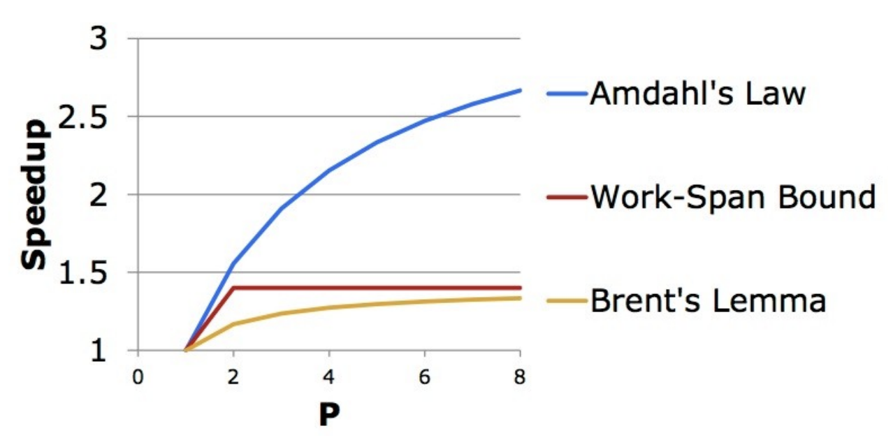
Lower/upper bound on greedy scheduling

• suppose we only have $P$ workers
• we can write a work-span formula to derive a lower bound on $T_P$ → $Max(T_1/P,T_{\infty })\le T_P$
• $T_{\infty }$ is the best possible execution time
• Brent’s Lemma derives an upper bound:
  • capture the additional cost executing the other tasks not on the critical path
  • assume we can do so without overhead
  • $T_P\le (T_1-T_{\infty })/P+T_{\infty }$

Amdahl was an optimist

Note

kind of ended slide 31? he speedran through the rest

Midterm

• no multiple choice? potentially
• 4 or 5 questions
• format will come via email!!!!!!!!