COSC 3P71: Exam Notes

Agents

Agent definitions

• Agent: something that takes in information from its surroundings (sensors) and does something in response (actuators)
• Agent function: rule or process that tells an agent what actions to take
• Agent program: the actual implementation of the agent function
• Percept: agent sensor input (text, images, sounds, etc.)
• Percept sequence: chatgpt history (history of what the agent has had as inputs)
• Rational: reasonably correct (does not need to be perfect), depends on 4 things:
  1. performance measure
  2. agent’s prior knowledge of the environment
  3. actions the agent can perform
  4. percept history to date
• Rational agent: an agent that selects the action that maximizes performance measure (“does the right thing”)
• Performance measure: a way to judge how well an agent is doing its job (e.g. chess game → win rate, self driving car → reaching destination safely and quickly, recommendation system → how often users click/like suggestions)
• PEAS framework:
  • Performance measure
  • Environment: the surroundings the agent operates in
  • Actuators: the parts that lets the agent take action (wheels, arms, display, …)
  • Sensors: the parts that let the agent perceive or gather information (camera, microphone, GPS, …)

Environment types:

• Fully observable vs partially observable
  • Fully observable: agent can see everything it needs to make a decision (e.g. chess)
  • Partially observable: agent only sees part of the environment (e.g. driving in fog)
• Deterministic vs stochastic
  • Deterministic: the next state is completely determined by the current state and action (no randomness)
  • Stochastic: there is some randomness in what happens next
• Episodic vs sequential
  • Episodic: each action is independent → what you do now doesn’t effect the next (e.g. image recognition)
  • Sequential: actions build on each other, past decisions matter (e.g. chess, driving)
• Static vs dynamic
  • Static: environment doesn’t change while the agent is thinking (e.g. crossword puzzle, sudoku)
  • Dynamic: environment changes over time, even if the agent is not acting (e.g. real world, driving)
• Discrete vs continuous
  • Discrete: limited number of possible states (e.g. chess, other board games)
  • Continuous: states and actions can take any value (e.g. driving speed, robot arm angles)
• Single vs multi agent
  • Single-agent: only one agent is acting (e.g. solving a maze)
  • Multi-agent: multiple agents interact, possibly competing or cooperating (e.g. soccer, trading bots)

Agent types

• Simple reflex agent: acts only based on current situation, uses conditional rules

  • only works in fully observable environments

• Model-based reflex agent: keeps some internal memory (model) of the world, uses current input and past information to decide what to do

  • used in partially observable environments

• Goal-based agent: has specific goals it tries to achieve, can plan ahead and compare different possible outcomes

• Problem-solving agent: a type of goal-based agent that uses search and planning to find a way to reach its goal

  • Problem-solving cycle:
    1. goal formulation → define desirable states
    2. problem formulation → identify states and actions relevant to goal
    3. search → find sequences of actions that reach goal
    4. execution → carry out actions — Utility-based agent: tries to maximize performance, uses utility function to measure how good each action is
  • utility: numerical value representing how desirable an outcome is; utility-based agents choose actions with highest expected utility

• Learning agent: improves over time by learning from experience

Genetic Algorithms

Darwinian Evolution Principles

• Survival of the fittest: resources are limited, only the most adaptable individuals reproduce, selection ensures only efficient competitors survive
• Diversity drives change:
  • behavioural/physical differences are partly inherited, partly random
  • traits increasing reproduction chances and heritable → spread over generations
  • leads to new combinations and evolutions of species
• Population dynamics:
  • population = unit of evolution
  • individual = unit of selection
  • random variations + selection = constant diversity source
  • no guiding force → evolution is emergent, not directed

Natural & biological evolution

• Alleles: possible values of a gene
• Chromosomes: long DNA molecules containing many genes
• Genome: complete genetic material
• Genotype: gene set of an individual
• Phenotype: observable characteristics from genotype
• Key conditions for evolution:
  • Reproduction with inheritance: individuals make copies of themselves
    • copies should resemble their parents (not be duplicates)
  • Variation: ensure that copies are not identical to parents
    • mutations, crossover produces individuals with different traits
  • Selection: need a method to ensure that some individuals make copies of themselves more than others
    • fittest individuals (favourable traits) have more offspring than unfit individuals, and population therefore has those traits
    • over time, changes will cause new species that can specialize for particular environments

Genetic Algorithms

Natural Concept	Genetic Algorithm Equivalent
Chromosome	solution representation
Gene	feature or variable
Allele	feature falue
Locus	gene position
Genotype	encoded structure (solution encoding)
Phenotype	decoded solution (actual parameters)

Main steps

1. Initialization: generate initial population
2. Evaluation: compute fitness for each solution
3. Selection: choose individuals for reproduction
4. Crossover: mix parents to create children
5. Mutation: introduce random variations
6. Replacement: update population for next generation
7. Termination: stop when condition met (e.g. max generations, target fitness hit)

Key variants

• Simple GA (SGA): full population replaced each generation
• Steady-state GA: only a few individuals replaced each iteration
• elitism: copy a few best individuals unchanged into the next generation so high-fitness solutions are preserved

Selection methods

• Tournament selection: select $k$ random individuals and keep the best for reproduction, repeat until you have a chosen amount of parents
• Roulette wheel selection: probabilistic selection based on fitness, $P(i)=\frac{f(i)}{{\sum }_{j=1}^{n}f(j)}$

Premature Convergence

• the population consists of similar individuals, it reduces likelihood of finding new solutions

Genetic Operators

• Crossover: a method of combining two candidates from. the population to create new candidates
• Mutation: lets offspring evolve in new directions → introduces a certain amount of randomness (certain traits may become fixed)
• Replication: copy an individual

Crossover Operations

• 1-point crossover:

Step 1: Choose random crossover point
P1:  1  2  3  |  4  5  6  7
P2:  7  6  5  |  4  3  2  1
              ↑ crossover point

Step 2: Swap segments after crossover point
C1:  1  2  3  |  4  3  2  1
C2:  7  6  5  |  4  5  6  7

✅ Final Offspring  
C1: 1  2  3  4  3  2  1  
C2: 7  6  5  4  5  6  7

• 2-points crossover:

Step 1: Choose two random crossover points
P1:  1  2 | 3  4  5 | 6  7
P2:  7  6 | 5  4  3 | 2  1
          ↑         ↑
         crossover points

Step 2: Swap middle segments between parents
C1:  1  2 | 5  4  3 | 6  7
C2:  7  6 | 3  4  5 | 2  1

✅ Final Offspring  
C1: 1  2  5  4  3  6  7  
C2: 7  6  3  4  5  2  1

• Uniform crossover (UX): each gene has a 50% chance of being inherited from either parent

Step 1: Generate random mask
P1:   1  2  3  4  5  6  7
Mask: 1  0  1  0  0  1  0
P2:   7  6  5  4  3  2  1

Step 2: Copy by mask (1 → from P1, 0 → from P2)
C1:   1  6  3  4  3  6  1
C2:   7  2  5  4  5  2  7

✅ Final Offspring  
C1: 1 6 3 4 3 6 1  
C2: 7 2 5 4 5 2 7

• Order crossover (OX):
  1. copying a randomly selected set from the first parent
  2. filling the remaining positions with the order of elements from the second

Step 1: Copy randomly selected set from first parent  
p1: 1 2 3 4 5 6 7 8 9  
p2: 9 3 7 8 2 6 5 1 4  

c1: * * * 4 5 6 7 * *  
c2: * * * 8 2 6 5 * *  

Step 2: Copy rest from second parent in order  
Remaining order from p2: 1, 9, 3, 8, 2  

C1: 3 8 2 4 5 6 7 1 9  
C2: ?

Step 1: Copy randomly selected set from first parent  
p1: 1 2 3 4 5 6 7 8 9  
p2: 4 5 2 1 8 7 6 9 3  

c1: * * * 4 5 6 7 * *  

Step 2: Copy rest from second parent in order  
Remaining order from p2: 9, 3, 2, 1, 8  

C1: 2 1 8 4 5 6 7 9 3  

• Uniform order crossover (UOX):

Step 1: Setup  
Parents (P1, P2) and Mask  
P1:   6  2  1  4  5  7  3  
Mask: 0  1  1  0  1  0  1  → generate new mask for every 2 parents
P2:   4  3  7  2  1  6  5  

Step 2: Copy Genes by Mask  
- Copy genes from P1 → C1 where mask = 1  
- Copy genes from P2 → C2 where mask = 1  

C1:   -  2  1  -  5  -  3  
C2:   -  3  7  -  1  -  5  

Step 3: Fill Remaining from Opposite Parent  
- Fill blanks (-) with remaining genes from the other parent in order  

C1:   4  2  1  7  5  6  3  
C2:   6  3  7  2  1  4  5  

✅ Final Offspring  
C1:  4  2  1  7  5  6  3  
C2:  6  3  7  2  1  4  5  

• Partially mapped crossover (PMX): preserves relative order and position (used for permutation problems)

Step 1: Select two crossover points
P1:  1  2 | 3  4  5 | 6  7  8
P2:  4  5 | 6  7  8 | 1  2  3

Step 2: Copy middle section from P1 → C1
C1:  *  * | 3  4  5 | *  *  *

Step 3: Map remaining genes from P2 using the mapping of swapped section
Mapping: 3↔6, 4↔7, 5↔8

Fill remaining using P2 order, applying mapping:
P2 order: 4 5 6 7 8 1 2 3  
→ Apply mapping to avoid duplicates

✅ Final Offspring  
C1:  6  7 | 3  4  5 | 8  1  2

• Cycle crossover (CX): every gene comes from one parent in the same same index across cycles

Step 1: Find cycles based on position mapping
P1:  1  2  3  4  5  6  7
P2:  3  7  5  1  6  2  4

Mapping:  
1 → 3 (pos3) → 5 (pos5) → 6 (pos6) → 2 (pos2) → 7 (pos7) → 4 (pos4) → 1  
Cycle: (1,3,5,6,2,7,4)

Step 2: Copy first cycle from P1, rest from P2
C1:  1  2  3  4  5  6  7
C2:  3  7  5  1  6  2  4

✅ Final Offspring  
C1: 1  2  3  4  5  6  7  
C2: 3  7  5  1  6  2  4

Mutation

• Inversion: reversed order of selected segment of genes

9 3 7 8 2 6 5 1 4 → 9 3 6 2 8 7 5 1 4

• Insertion: select one gene and insert it into a random position

9 3 7 8 2 6 5 1 4 → 9 7 8 2 3 6 5 1 4

• Displacement: select a subtour (continuous segment) and reinsert it somewhere else

9 3 7 8 2 6 5 1 4 → 9 8 2 6 5 3 7 1 4

• Reciprocal exchange (swap): select two genes and swap their positions

9 3 7 8 2 6 5 1 4 → 5 3 7 8 2 6 9 1 4

• Scramble mutation: select a subset of genes and randomly shuffle their order

9 3 7 8 2 6 5 1 4 → 9 3 6 8 7 2 5 1 4

EVERYTHING ABOVE IS PRE-MIDTERM

Games (Adversarial Search)

• adversarial, multi-agent environments (MAX vs MIN)

• defined by: initial state, legal moves, terminal test, utility

• game tree → nodes = states, edges = moves, ply = depth layer

• full search often impossible → rely on heuristics + cutoff

• what makes a game different from normal search?:

  • multi-agent, competitive, adversarial
  • opponent affects your outcome
  • need a strategy, not just a path
  • goal: choose actions that maximize your payoff against an optimal opponent

Minimax

• idea:
  • perfect play under deterministic, perfect-information games
  • MAX chooses move with the highest worst-case value
  • assume opponent is rational and tries to minimize your score
• procedure:
  1. expand game tree to some depth
  2. evaluate leaf nodes with evaluation function
  3. back up values:
     • MAX nodes take max of children
     • MIN nodes take min of children
  4. choose best move at root
• properties:
  • complete (if tree finite)
  • optimal (against optimal opponent)
  • expensive: $O(b^m)$ time, $O(b^m)$ space

Alpha-beta pruning

• purpose:
  • avoid evaluating branches that cannot affect the final decision
  • works alongside minimax → same final answer, faster search
• key ideas:
  • $\alpha$ (alpha): best score MAX can guarantee so far
  • $\beta$ (beta): best score MIN can guarantee so far
  • if a branch is already worse than what a player can get elsewhere → prune it
• benefits:
  • eliminates huge parts of tree
  • with good move ordering, reduces time from $O(b^m)$ to $O(b^{(}m/2))$
  • allows deeper search within the same time

Evaluation functions

• used when search is cut off early
• heuristic score estimating “how good” a state is
• usually weighted sum of features
• must correlate with probability of winning

Cutoff search

• search only to fixed depth (resource limits)
• evaluate non-terminal states using evaluation function
• risk: horizon effect (bad events hidden beyond depth)

Search enhancements

• iterative deepening: search 1 ply, then 2, then 3.. until time expires
• quiescence search: extend search in volatile positions (captures, threats)
• move ordering: improves alpha-beta effectiveness
• singular extension: explore unusually promising moves deeper

Swarm Intelligence

Ant Colony Optimization (ACO)

• population-based stochastic (some randomness) search using ants and pheromone
• ants choose edges probabilistically based on pheromone + visibility
• positive feedback: good paths get reinforced
• evaporation: keeps pheromone from exploding → forces exploration
• loop: create ants → build solution → evaporate → add pheromone
• needs graph representation; finite path
• issues: converges fast

Particle Swarm Optimization (PSO)

• swarm of particles moving in search space
• each particle has position and velocity
• particles remember:
  • personal best (pbest)
  • global best (gbest)
• velocity updated using:
  • momentum (old velocity)
  • pull toward pbest
  • pull toward gbest
• movement influenced by randomness → exploration
• fast convergence but may get stuck if swarm collapses early

Learning & Machine Learning

• machine learning: programs that improve with experience

• Mitchell’s definition: learns if performance on task T improves using experience E measured by P

• checkers ML example (T/P/E):

  • Task (T): play checkers
  • Performance (P): % games won
  • Experience (E): games of self-play used as training data

• types of learning

  • supervised: labeled data (classification, regression)
  • unsupervised: no labels (clustering)
  • reinforcement: reward-based learning
  • exploration vs exploitation: balance between trying new actions to gather information vs using known high-reward actions

• supervised examples: decision tree classifier, perceptron/NN classifier

• unsupervised examples: k-means, hierarchical clustering

Designing a learning system

• choose training experience
• choose target function
• choose representation (rules, tables, linear model, neural networks)
• choose learning algorithm (e.g. gradient descent)

Memorization vs generalization

• memorization: model stores training examples, performs poorly on new data
• generalization: model learns underlying patterns, performs well on unseen data
• overfitting: too much memorization, not enough generalization

Training experience issues

• must be representative (training examples must reflect real situations the agent will face)
  • e.g. if a spam filter is trained on only old emails, it won’t generalize to modern spam
• feedback may be direct (correct answer provided) or indirect (reinforcement → only rewards or signals)
• may or may not involve a teacher (provided correct labels vs learner must find structure)
  • e.g. clustering animals without knowing categories
• bad data (noisy, biased, incomplete, incorrect labelling, …) harms performance

ML challenges

• model complexity:
  • too simple → underfitting (can’t capture patterns)
  • too complex → overfitting (memorizes training data)
• training data size: more data → generally better performance, too little → poor generalization
• noise in data: incorrect labels or irrelevant features degrade accuracy
• learnability limits: some things are inherently hard to learn
  • e.g. predicting stock price → hard due to chaotic signals
• prior knowledge: using domain knowledge can constrain hypotheses and improve learning
  • e.g. knowing legal moves in chess reduces search space → better performance

Decision Trees & Overfitting

Decision trees

• supervised learning method for classification
• recursively split data based on attributes
• internal nodes = tests; branches = outcomes; leaves = class labels
• good for data with clear, rule-line data
• handles discrete or continuous attributes (continuous → threshold tests)

How to build one

• choose attribute that best separates data
• common criteria:
  • information gain (IG): reduction in entropy (uncertainty) after a split
  • gain ratio: normalizes IG by attribute branching factor
• repeat splitting on subsets until:
  • all examples in node have same class
  • no attributes left
  • data too small

Advantages

• interpretable (human-readable rules)
• fast to train
• little data preprocessing required
• can capture non-linear boundaries

Disadvantages

• unstable (small data changes → different tree)
• greedy splitting may miss globally optimal tree
• prone to oversplitting
• optimal tree size: finding the smallest decision tree is NP-hard → practical algorithms use greedy heuristics instead of exhaustive search

Overfitting (in decision trees)

• model becomes too specific to training data
• memorizes noise instead of learning patterns
• tree grows too deep with many small, impure leaves

Signs of overfitting

• high accuracy on training data & low accuracy on unseen data
• branches based on rare or noisy attribute combinations

Causes

• noisy data
• too many attributes
• insufficient training examples
• splitting until leaves are tiny (one or few samples)

Preventing overfitting

• pre-pruning: stop early
  • limit tree depth
  • minimum samples per node
  • require split to exceed IG threshold
• post-pruning: build full tree, then trim
  • remove branches that do not improve validation accuracy
  • replaces overfitted subtrees with leaf nodes
• cross-validation: ensures splits generalize
• simplify attributes: remove irrelevant features

Neural Networks

• model made of neurons connected by weighted edges
• each neuron: sum of inputs → apply activation function → output
• learning = adjusting weights so outpus match targets

Perceptron (single layer network)

• linear classifier (straight line decision boundary)
• works only for linearly separable problems
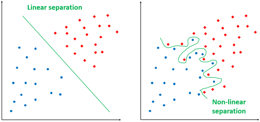
• weight update rule reduces classification error
• limit: cannot learn XOR or any non-linear separation

Why multilayer networks?

• add hidden layers → can learn non-linear functions
• input → hidden (can be multiple) → output
• hidden units combine features → represent complex patterns

Activation functions

• a rule that transforms a neuron’s summed input into its output, adding the non-linearity needed for neural networks to learn complex patterns
• common forms:
  • step/sign function: perceptron-style (not differentiable, not usable for backprop)
  • sigmoid/tanh: smooth, differentiable → needed for backprop
• choice affects learning speed + representational power

Training neural networks

• forward pass:
  • input flows through layers to produce prediction
• back-propagation (error-correcting learning):
  • compare prediction to target → compute error
  • send error backwards through network
  • adjust weights using gradient descent
  • requires differentiable activation functions
• intuition:
  • if output is wrong → adjust weights that contributed to error
  • small learning rate = stable but slow
  • large learning rate = fast but unstable

Strengths

• learns complex, non-linear patterns (multi-layer)
• good for classification, pattern recognition, noisy data
• no need for explicit rules → model “discovers” structure

Limitations

• weights are a black box → poor interpretability
• can overfit (memorize training data)
• needs lots of data + careful tuning
• training may get stuck in local minima (gradient descent)

Clustering

• unsupervised learning: group similar data points without labels
• goal: high similarity within clusters, low similarity between different clusters
• works only if real structure exists in data
• results must be interpreted → algorithm will always produce clusters, even if meaningless
• examples: images, patterns, documents, shopping items, biological data, social networks

Hierarchical clustering

• builds a tree of nested clusters
• no need to pick the number of clusters beforehand
• two types:
  • agglomerative: start with each point alone → repeatedly merge closest clusters
  • divisive: start with all points together → repeatedly split

Linkage criteria (how to measure distance between clusters):

• single linkage: nearest points → long “chain-like” clusters
• complete linkage: farthest points → compact clusters
• average linkage: average distance → balances sensitivity
• centroid linkage: distance between cluster centroids

Limitations

• early merge/split decisions cannot be undone
• choosing where to “cut” the tree is subjective

Partitioning clustering

• choose $k$ (number of clusters) first
• assign points to clusters based on similarity to representatives

K-means

• most common partitioning clustering method
• tries to minimize distances between points and their cluster centers (centroids)

How it works

• pick $k$ initial centers
• assign each point to nearest center
• recompute centers
• repeat until stable

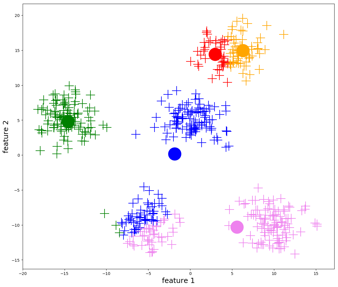
Strengths

• simple, fast, handles large datasets
• can adjust assignments if initial choices were bad

Weaknesses

• sensitive to initial needs
• not guaranteed to find the optimal clustering
• must choose $k$ manually
• can get stuck in local minima

Validation

• why validate?: clustering always produces groups → need to check if they’re meaningful
• ways to validate:
  • internal: based on cluster quality (tightness, separation)
  • external: compare to known labels or external variables
  • relative: compare results across different $k$ values or algorithms

Common difficulties

• choosing the right number of clusters
• noise and outliers distort cluster structure
• results depend heavily on distance measure
• hard to visualize high-dimensional clusters
• multiple valid clusterings may exist for the same dataaf

Logic

Common Logic Symbols

Symbol	Meaning	Example	Plain English Explanation
$\neg$	not	$\neg P$	”Not P” → P is false
$\wedge$	and	$P\wedge Q$	P and Q are both true
$\vee$	or (inclusive)	$A\vee B$	At least one of A or B is true
$\to$	implies	$P\to Q$	If P is true, then Q must also be true
$\leftrightarrow$	biconditional (iff)	$P\leftrightarrow Q$	P is true exactly when Q is true
$=$	equality	$x=y$	x and y are the same object/value
$\forall$	universal quantifier (“for all”)	$\forall xLoves(x,Pizza)$	Everybody loves pizza
$\exists$	existential quantifier (“there exists”)	$\exists xStudent(x)$	At least one student exists
$Predicate(term)$	relation between objects	$Friends(Alice,Bob)$	Alice and Bob are friends
Function$(x)$	returns an object	$FatherOf(John)$	”John’s father”
Variables	placeholders for objects	$P(x)$	P applies to some object x

Knowledge Representation (KR)

• express knowledge in a form the agent can use
• good KR: explicit, concise, suppresses irrelevant detail, supports reasoning

Logic basics

• syntax: structure of a sentence
• semantics: truth in a model
• entailment: $\text{KB}\models (\alpha \to \alpha )$ in all models of KB
• inference: derive new sentences; must be sound and complete

Propositional Logic (PL)

• simple true/false statements combined with $\neg$, $\wedge$, $\vee$, $\to$, $\leftrightarrow$
• truth tables define semantics
• strength: simple, compositional
• weakness: cannot talk about objects/relations; low expressive power

Propositional Logic (PL) Examples

• $P\wedge Q$
  • Meaning: It is raining and it is cold.
  • $P$: “It is raining”
  • $Q$: “It is cold”
• $\neg R\to S$
  • Meaning: If the door is not locked, then the alarm is on.
  • $R$: “The door is locked”
  • $S$: “The alarm is on”
• $(A\vee B)\wedge \neg C$
  • Meaning: Lights are on or motion is detected, and there is no power failure.
  • $A$: “Lights are on”
  • $B$: “Motion detected”
  • $C$: “Power failure”

First-Order Logic (FOL)

• adds objects, relations, functions, variables, quantifiers
• much more expressive than PL

First-Order Logic (FOL) Examples

• $\forall x(Student(x)\to Smart(x))$
  • Meaning: Every student is smart.
• $\exists yLoves(John,y)$
  • Meaning: John loves at least one person.
• $Brother(Richard,John)\wedge King(John)$
  • Meaning: Richard is John’s brother, and John is a king.

FOL "at Google" patterns

• $\forall x(AtGoogle(x)\to Smart(x))$
  • Meaning: Everyone at Google is smart.
• $\forall xAtGoogle(x)\wedge \forall xSmart(x)$
  • Meaning: Everyone is at Google, and everyone is smart.
• $\exists x(AtGoogle(x)\wedge Smart(x))$
  • Meaning: Someone at Google is smart.

Quantifiers

• universal: $\forall xP(x)$ → “for all x”
  • correct pattern: $\forall x(A(x)\to B(x))$
• existential: $\exists xP(x)$ → “there exists x”
  • correct pattern: $\exists x(A(x)\wedge B(x))$
• quantifier properties:
  • $\forall$ and $\exists$ commute with themselves, not with each other
  • duality:
    • $\forall xP\equiv \neg \exists x\neg P$
    • $\exists xP\equiv \neg \forall x\neg P$

PL vs FOL

Feature	PL	FOL
talks about	facts	objects + relations
variables	no	yes
quantifiers	no	$\forall$, $\exists$
expressiveness	low	high

• implication equivalence: (X \rightarrow Y \equiv \neg X \lor Y) (tautology)

Philosophy & AI

Core questions

• what is a mind? how do human minds work?
• can non-human systems (like computers) have minds?
• what counts as thinking or understanding?

Weak & strong AI

• weak AI: AI produces useful tools and intelligent behaviour, but not real understanding or minds
• strong AI: a machine can literally have a mind, understanding, intentions, consciousness
• arguments raised against strong AI:
  • some tasks may be impossible for computers, no matter how we program them
  • certain designs of “intelligent programs” fail inherently
  • programs may simulate intelligence without truly understanding
  • practical limits: complexity, infeasibility of encoding full human cognition

Turing Test

• idea: if a machine can hold a conversation indistinguishable from a human, treat it as intelligent
• strengths:
  • avoids metaphysical debates (“can machines think?”)
  • focuses on observable behaviour
• critiques:
  • measures performance, not inner understanding
  • easy to foot naive interrogators
  • does not assess reasoning, emotion, self-awareness
  • machine may pass via tricks, not intelligence
• famous turing test objections:
  • lovelace objection: machines cannot originate anything → they do what we tell them
  • species-centricity: assumes humans must be more intelligent
  • mathematical objection: godel style limits → formal systems cannot solve everything
  • onsciousness objection: intelligence requires awareness, emotions, subjective experience
  • diversity objection: humans vary widely; programs may not

Chinese room argument

• setup:
  • person (doesn’t know chinese) goes in a room
  • given chinese text (paragraphs) and questions, rules describing how to manipulate Chinese symbols from questions and text, and output corresponding Chinese text
  • person is being the “computer processor”
  • chinese room = syntax $\ne$ semantics; programs don’t understand
• claim:
  • running a program (symbol manipulation) is not enough for understanding or intentionality
  • strong AI is false: programs do not genuinely “understand” even if they behave correctly
• counterarguments:
  • systems reply: the whole system understands, not the person
  • brain simulator reply: simulating neural processes would produce understanding
  • many mansions reply: non-digital mechanisms might produce real cognition
  • robot reply (implied): embodiment may be required for meaning